Tutorial training F32

This tutorial should explain how the different components of AIfES 2 work together to train a simple Feed-Forward Neural Network (FNN) or Multi Layer Perceptron (MLP). If you just want to perform an inference with pretrained weights, switch to the inference tutorial.

Example

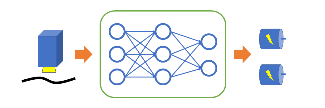
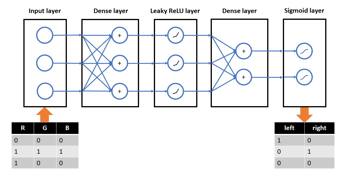
As an example, we take a robot with two powered wheels and a RGB color sensor that should follow a black line on a white paper. To fulfill the task, we map the color sensor values with an FNN directly to the control commands for the two wheel-motors of the robot. The inputs for the FNN are the RGB color values scaled to the interval [0, 1] and the outputs are either "on" (1) or "off" (0) to control the motors.

The following cases should be considered:

1. The sensor points to a black area (RGB = [0, 0, 0]): The robot is too far on the left and should turn on the left wheel-motor while removing power from the right motor.
2. The sensor points to a white area (RGB = [1, 1, 1]): The robot is too far on the right and should turn on the right wheel-motor while removing power from the left motor.
3. The sensor points to a red area (RGB = [1, 0, 0]): The robot reached the stop mark and should switch off both motors.

The resulting input data of the FNN is then

R	G	B
0	0	0
1	1	1
1	0	0

and the output should be

left motor	right motor
1	0
0	1
0	0

Design the neural network

To set up the FNN in AIfES 2, we need to design the structure of the neural network. It needs three inputs for the RGB color values and two outputs for the two motors. Because the task is rather easy, we use just one hidden layer with three neurons.

To create the network in AIfES, it must be divided into logical layers like the fully-connected (dense) layer and the activation functions. We choose a Leaky ReLU activation for the hidden layer and a Sigmoid activation for the output layer.

Create the neural network in AIfES

AIfES provides implementations of the layers for different data types that can be optimized for several hardware platforms. An overview of the layers that are available for training can be seen in the overview section of the main page. In the overview table you can click on the layer in the first column for a description on how the layer works. To see how to create the layer in code, choose one of the implementations for your used data type and click on the link.
In this tutorial we work with the float 32 data type (F32 ) and use the default implementations (without any hardware specific optimizations) of the layers.

Used layer types:

• Input layer
• Dense layer
• Leaky ReLU layer
• Sigmoid layer

Used implementations:

• ailayer_input_f32_default()
• ailayer_dense_f32_default()
• ailayer_leaky_relu_f32_default()
• ailayer_sigmoid_f32_default()

Declaration and configuration of the layers

For every layer we need to create a variable of the specific layer type and configure it for our needs. See the documentation of the data type and hardware specific implementations (for example ailayer_dense_f32_default()) for code examples on how to configure the layers.

Our designed network can be declared with the following code

// The main model structure that holds the whole neural network
aimodel_t model;
 
 
// The layer structures for F32 data type and their configurations
uint16_t input_layer_shape[] = {1, 3};
ailayer_input_f32_t input_layer           = AILAYER_INPUT_F32_A(2, input_layer_shape);
ailayer_dense_f32_t dense_layer_1         = AILAYER_DENSE_F32_A(3);
ailayer_leaky_relu_f32_t leaky_relu_layer = AILAYER_LEAKY_RELU_F32_A(0.01f);
ailayer_dense_f32_t dense_layer_2         = AILAYER_DENSE_F32_A(2);
ailayer_sigmoid_f32_t sigmoid_layer       = AILAYER_SIGMOID_F32_A();

We use the initializer macros with the "_A" at the end, because we call aialgo_distribute_parameter_memory() later on to set the remaining paramenters (like the weights) automatically.

Connection and initialization of the layers

Afterwards the layers are connected and initialized with the data type and hardware specific implementations

// Layer pointer to perform the connection
ailayer_t *x;
 
model.input_layer = ailayer_input_f32_default(&input_layer);
x = ailayer_dense_f32_default(&dense_layer_1, model.input_layer);
x = ailayer_leaky_relu_f32_default(&leaky_relu_layer, x);
x = ailayer_dense_f32_default(&dense_layer_2, x);
x = ailayer_sigmoid_f32_default(&sigmoid_layer, x);
model.output_layer = x;
 
// Finish the model creation by checking the connections and setting some parameters for further processing
aialgo_compile_model(&model);

Set the memory for the trainable parameters

Because AIfES doesn't allocate any memory on its own, you have to set the memory buffers for the trainable parameters like the weights and biases manually. Therefore you can choose fully flexible, where the parameters should be located in memory. To calculate the required amount of memory by the model, the aialgo_sizeof_parameter_memory() function can be used or the size can be calculated manually (See the sizeof_paramem() functions of every layer for the required amount of memory and the set_paramem() function for how to set it to the layer).
With aialgo_distribute_parameter_memory() a memory block of the required size can be distributed and set to the different trainable parameters of the model.

A dynamic allocation of the memory using malloc could look like the following:

uint32_t parameter_memory_size = aialgo_sizeof_parameter_memory(&model);
void *parameter_memory = malloc(parameter_memory_size);
 
// Distribute the memory to the trainable parameters of the model
aialgo_distribute_parameter_memory(&model, parameter_memory, parameter_memory_size);

You could also pre-define a memory buffer if you know the size in advance, for example

const uint32_t parameter_memory_size = 80;
char parameter_memory[parameter_memory_size];
 
...
 
// Distribute the memory to the trainable parameters of the model
aialgo_distribute_parameter_memory(&model, parameter_memory, parameter_memory_size);

Print the layer structure to the console

To see the structure of your created model, you can print a model summary to the console

aiprint("\n-------------- Model structure ---------------\n");
aialgo_print_model_structure(&model);
aiprint("----------------------------------------------\n\n");

Train the neural network

The created FNN can now be trained. AIfES provides the necessary functions to train the model with the backpropagation algorithm.

Configure the loss

To calculate the gradients for the backpropagation training algorithm, a loss function must be configured to the model. An overview of available losses can be seen in the overview section of the main page. In the overview table you can click on the loss in the first column for a description on how the loss works. To see how to create the loss in code, choose one of the implementations for your used data type and click on the link.

In this tutorial we work with the float 32 data type (F32 ) and use the default implementation (without any hardware specific optimizations) of the loss. We choose the Cross-Entropy loss because we have sigmoid outputs of the network and binary target data. (Cross-Entropy loss will not work for other output layers than sigmoid or softmax!)

Used loss type:

• Cross-Entropy loss

Used implementation:

• ailoss_crossentropy_f32_default()

The loss can be declared, connected and initialized similar to the layers, by calling

ailoss_crossentropy_f32_t crossentropy_loss;
 
model.loss = ailoss_crossentropy_f32_default(&crossentropy_loss, model.output_layer);

You can print the loss configuration to the console for debugging purposes with

aialgo_print_loss_specs(model.loss);

Configure the optimizer

To update the parameters with the calculated gradients, an optimizer must be created. An overview of available optimizers can be seen in the overview section of the main page. In the overview table you can click on the optimizer in the first column for a description on how the loss works. To see how to create the optimizer in code, choose one of the implementations for your used data type and click on the link.

In this tutorial we work with the float 32 data type (F32 ) and use the default implementation (without any hardware specific optimizations) of the optimizer. We choose the Adam optimizer that converges really fast to the optimum with just a small memory and computation overhead. On more limited systems, the SGD optimizer might be a better choice.

Used optimizer type:

• Adam optimizer

Used implementation:

• aiopti_adam_f32_default()

The optimizer can be declared and configured by calling

aiopti_adam_f32_t adam_opti = {
    .learning_rate = 0.01f,
 
    .beta1 = 0.9f,
    .beta2 = 0.999f,
    .eps = 1e-7f
};

in C or

aiopti_adam_f32_t adam_opti = AIOPTI_ADAM_F32(0.01f, 0.9f, 0.999f, 1e-7f);

in C++ and on Arduino. Afterwards it can be initialized by

aiopti_t *optimizer = aiopti_adam_f32_default(&adam_opti);

You can print the optimizer configuration to the console for debugging purposes with

aialgo_print_optimizer_specs(optimizer);

Initialize the trainable parameters

The trainable parameters like the weights and biases have to be initialized before the training. There are different initialization techniques for different models. For a simple FNN, the recommended initialization of the weights and biases of the dense layers are dependent on the connected activation functions

Activation function	Weights-init	Bias-init
None, tanh, sigmoid, softmax	Glorot	Zeros
ReLU and variants	He	Zeros
SELU	LeCun	Zeros

In our example, the two dense layers can be initialized manually like described in the recommendation table (uniform distribution versions)

// Set the seed for your configured random function for example with
srand(time(0));
 
aimath_f32_default_init_he_uniform(&dense_layer_1.weights);
aimath_f32_default_init_zeros(&dense_layer_1.bias);
 
aimath_f32_default_init_glorot_uniform(&dense_layer_2.weights);
aimath_f32_default_init_zeros(&dense_layer_2.bias);

AIfES can also automatically initialize the trainable parameters of the whole model with the default initialization methods configured to the layers.

// Set the seed for your configured random function for example with
srand(time(0));
aialgo_initialize_parameters_model(&model);

Allocate and initialize the working memory

Because AIfES doesn't allocate any memory on its own, you have to set the memory buffers for the training manually. This memory is required for example for the intermediate results of the layers, for the gradients and as working memory for the optimizer (for momentums). Therefore you can choose fully flexible, where the buffer should be located in memory. To calculate the required amount of memory for the training, the aialgo_sizeof_training_memory() function can be used.
With aialgo_schedule_training_memory() a memory block of the required size can be distributed and scheduled (memory regions might be shared over time) to the model.

A dynamic allocation of the memory using malloc could look like the following:

uint32_t training_memory_size = aialgo_sizeof_training_memory(&model, optimizer);
void *training_memory = malloc(training_memory_size);
 
// Schedule the memory to the model
aialgo_schedule_training_memory(&model, optimizer, training_memory, training_memory_size);

You could also pre-define a memory buffer if you know the size in advance, for example

const uint32_t training_memory_size = 772;
char training_memory[training_memory_size];
 
...
 
// Schedule the memory to the model
aialgo_schedule_training_memory(&model, optimizer, training_memory, training_memory_size);

Before starting the training, the scheduled memory must be initialized. The initialization sets for example the momentums of the optimizer to zero.

aialgo_init_model_for_training(&model, optimizer);

Perform the training

To perform the training, the input data and the target data / labels (and also the test data if available) must be packed in a tensor to be processed by AIfES. A tensor in AIfES is just a N-dimensional array that is used to hold the data values in a structured way. To do this, create 2D tensors of the used data type. The shape describes the size of the dimensions of the tensor. The first dimension (the rows) is the batch dimension, i.e. the dimension of the different training samples. The second dimension equals the inputs / outputs of the neural network.

uint16_t x_train_shape[2] = {3, 3};
float x_train_data[3*3] = {0.0f, 0.0f, 0.0f,
                           1.0f, 1.0f, 1.0f,
                           1.0f, 0.0f, 0.0f};
aitensor_t x_train = AITENSOR_2D_F32(x_train_shape, x_train_data);
 
// Target data / Labels for training
uint16_t y_train_shape[2] = {3, 2};
float y_train_data[3*2] = {1.0f, 0.0f,
                           0.0f, 1.0f,
                           0.0f, 0.0f};
aitensor_t y_train = AITENSOR_2D_F32(y_train_shape, y_train_data);

Because in this case we are just interested in the outputs of the FNN on our training dataset, our test data is just the training data.

aitensor_t *x_test = &x_train;
aitensor_t *y_test = &y_train;

Now everything is ready to perform the actual training. AIfES provides the function aialgo_train_model() that performs one epoch of training with mini-batches. One epoch means that the model has seen the whole data ones afterwards. The function aialgo_calc_loss_model_f32() can be used to calculate the loss on the test data between the epochs.

An example training with these functions that trains the model for a pre-defined amount of epochs might look like this:

int epochs = 100;
int batch_size = 3;
int print_interval = 10;
 
float loss;
aiprint("\nStart training\n");
for(int i = 0; i < epochs; i++)
{
    // One epoch of training. Iterates through the whole data once
    aialgo_train_model(&model, &x_train, &y_train, optimizer, batch_size);
 
    // Calculate and print loss every print_interval epochs
    if(i % print_interval == 0)
    {
        aialgo_calc_loss_model_f32(&model, x_test, y_test, &loss);
        
        // Print the loss to the console
        aiprint("Epoch "); aiprint_int("%5d", i);
        aiprint(": test loss: "); aiprint_float("%f", loss);
        aiprint("\n");
    }
}
aiprint("Finished training\n\n");

If you like to have more control over the training process, you can also use the more advanced functions

• aialgo_zero_gradients_model()
• aialgo_forward_model()
• aialgo_backward_model()
• aialgo_update_params_model()

The call order of the functions in pseudo code could look like this

for epochs
    for each batch in dataset
        aialgo_zero_gradients_model()
        for each sample in the batch
            aialgo_forward_model()
            aialgo_backward_model()
        endfor
        aialgo_update_params_model()
    endfor
endfor

For a code example, see the source code of the aialgo_train_model() function.

Test the trained model

To test the trained model you can perform an inference on the test data and compare the results with the targets. To do this you can call the inference function aialgo_inference_model().

// Create an empty tensor for the inference results
uint16_t y_out_shape[2] = {3, 2};
float y_out_data[3*2];
aitensor_t y_out = AITENSOR_2D_F32(y_out_shape, y_out_data);
 
aialgo_inference_model(&model, x_test, &y_out);

Afterwards you can print the results to the console for further inspection:

aiprint("x_test:\n");
print_aitensor(x_test);
aiprint("NN output:\n");
print_aitensor(&y_out);

Change working memory

If you are satisfied with your trained model, you can delete the working memory created for the training (if it was created dynamically). For further inferences / usage of the model you should assign a new memory block, because the big training memory is not needed anymore. Use aialgo_schedule_inference_memory() to assign a (much smaller) memory block to the model that is made for inference. The required size can be calculated with aialgo_sizeof_inference_memory().

Example:

uint32_t inference_memory_size = aialgo_sizeof_inference_memory(&model);
void *inference_memory = malloc(inference_memory_size);
 
// Schedule the memory to the model
aialgo_schedule_inference_memory(&model, inference_memory, inference_memory_size);

Or

const uint32_t inference_memory_size = 24;
char inference_memory[inference_memory_size];
 
...
 
// Schedule the memory to the model
aialgo_schedule_inference_memory(&model, inference_memory, inference_memory_size);